Array Elements Must Be ________ Before a Binary Search Can Be Performed.

This article is about searching a finite sorted assortment. For searching continuous part values, see bisection method.

Search algorithm finding the position of a target value within a sorted assortment

Binary search algorithm

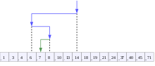Visualization of the binary search algorithm where 7 is the target value
Class	Search algorithm
Data construction	Array
Worst-example performance	O(log n)
Best-instance performance	O(1)
Average performance	O(log n)
Worst-case space complexity	O(1)

In computer science, binary search, also known as half-interval search,^[1] logarithmic search,^[2] or binary chop,^[iii] is a search algorithm that finds the position of a target value within a sorted array.^{[4] [5]} Binary search compares the target value to the middle element of the array. If they are not equal, the one-half in which the target cannot lie is eliminated and the search continues on the remaining half, again taking the middle element to compare to the target value, and repeating this until the target value is found. If the search ends with the remaining half existence empty, the target is not in the array.

Binary search runs in logarithmic time in the worst case, making ${\displaystyle O(\log n)}$ comparisons, where ${\displaystyle n}$ is the number of elements in the array.^{[a] [6]} Binary search is faster than linear search except for pocket-sized arrays. However, the array must be sorted commencement to be able to utilise binary search. At that place are specialized data structures designed for fast searching, such every bit hash tables, that can be searched more efficiently than binary search. However, binary search tin be used to solve a wider range of problems, such as finding the next-smallest or adjacent-largest element in the array relative to the target even if it is absent from the assortment.

There are numerous variations of binary search. In particular, fractional cascading speeds upwardly binary searches for the same value in multiple arrays. Fractional cascading efficiently solves a number of search problems in computational geometry and in numerous other fields. Exponential search extends binary search to unbounded lists. The binary search tree and B-tree data structures are based on binary search.

Algorithm [edit]

Binary search works on sorted arrays. Binary search begins by comparison an element in the middle of the array with the target value. If the target value matches the chemical element, its position in the array is returned. If the target value is less than the element, the search continues in the lower half of the array. If the target value is greater than the chemical element, the search continues in the upper half of the array. Past doing this, the algorithm eliminates the half in which the target value cannot lie in each iteration.^[vii]

Procedure [edit]

Given an array ${\displaystyle A}$ of ${\displaystyle n}$ elements with values or records ${\displaystyle A_{0},A_{1},A_{2},\ldots ,A_{n-1}}$ sorted such that ${\displaystyle A_{0}\leq A_{one}\leq A_{2}\leq \cdots \leq A_{n-1}}$ , and target value ${\displaystyle T}$ , the following subroutine uses binary search to find the index of ${\displaystyle T}$ in ${\displaystyle A}$ .^[7]

1. Set ${\displaystyle L}$ to ${\displaystyle 0}$ and ${\displaystyle R}$ to ${\displaystyle n-1}$ .
2. If ${\displaystyle L>R}$ , the search terminates as unsuccessful.
3. Set ${\displaystyle m}$ (the position of the middle element) to the floor of ${\displaystyle {\frac {L+R}{two}}}$ , which is the greatest integer less than or equal to ${\displaystyle {\frac {L+R}{2}}}$ .
4. If ${\displaystyle A_{one thousand}<T}$ , gear up ${\displaystyle L}$ to ${\displaystyle m+1}$ and become to step 2.
5. If ${\displaystyle A_{grand}>T}$ , set ${\displaystyle R}$ to ${\displaystyle 1000-one}$ and go to stride 2.
6. Now ${\displaystyle A_{m}=T}$ , the search is done; return ${\displaystyle yard}$ .

This iterative process keeps runway of the search boundaries with the 2 variables ${\displaystyle L}$ and ${\displaystyle R}$ . The procedure may exist expressed in pseudocode equally follows, where the variable names and types remain the same as above, floor is the flooring role, and unsuccessful refers to a specific value that conveys the failure of the search.^[vii]

          function          binary_search(A, due north, T)          is          L := 0     R := n − 1          while          L ≤ R          do          g := floor((50 + R) / ii)          if          A[m] < T          then          L := m + i          else if          A[m] > T          then          R := chiliad − 1          else:          return          1000          return          unsuccessful        

Alternatively, the algorithm may take the ceiling of ${\displaystyle {\frac {L+R}{two}}}$ . This may change the result if the target value appears more than than once in the array.

Alternative procedure [edit]

In the higher up process, the algorithm checks whether the heart element ( ${\displaystyle m}$ ) is equal to the target ( ${\displaystyle T}$ ) in every iteration. Some implementations leave out this check during each iteration. The algorithm would perform this cheque simply when one element is left (when ${\displaystyle L=R}$ ). This results in a faster comparison loop, as one comparing is eliminated per iteration, while information technology requires only one more iteration on average.^[8]

Hermann Bottenbruch published the get-go implementation to get out out this check in 1962.^{[8] [9]}

1. Gear up ${\displaystyle L}$ to ${\displaystyle 0}$ and ${\displaystyle R}$ to ${\displaystyle n-1}$ .
2. While ${\displaystyle Fifty\neq R}$ ,
   1. Prepare ${\displaystyle m}$ (the position of the middle chemical element) to the ceiling of ${\displaystyle {\frac {L+R}{2}}}$ , which is the least integer greater than or equal to ${\displaystyle {\frac {L+R}{2}}}$ .
   2. If ${\displaystyle A_{yard}>T}$ , prepare ${\displaystyle R}$ to ${\displaystyle yard-one}$ .
   3. Else, ${\displaystyle A_{grand}\leq T}$ ; prepare ${\displaystyle L}$ to ${\displaystyle m}$ .
3. At present ${\displaystyle 50=R}$ , the search is done. If ${\displaystyle A_{50}=T}$ , return ${\displaystyle Fifty}$ . Otherwise, the search terminates as unsuccessful.

Where ceil is the ceiling function, the pseudocode for this version is:

          function          binary_search_alternative(A, due north, T)          is          50 := 0     R := n − 1          while          Fifty != R          do          m := ceil((L + R) / ii)          if          A[m] > T          then          R := 1000 − one          else:             Fifty := m          if          A[L] = T          so          return          L          return          unsuccessful        

Indistinguishable elements [edit]

The process may return any index whose element is equal to the target value, fifty-fifty if there are duplicate elements in the array. For case, if the array to be searched was ${\displaystyle [ane,2,3,four,four,5,six,seven]}$ and the target was ${\displaystyle iv}$ , then information technology would be correct for the algorithm to either render the 4th (alphabetize 3) or 5th (alphabetize 4) element. The regular procedure would return the fourth element (index three) in this example. It does not ever return the commencement duplicate (consider ${\displaystyle [1,2,iv,4,4,five,vi,7]}$ which still returns the 4th element). However, information technology is sometimes necessary to find the leftmost chemical element or the rightmost element for a target value that is duplicated in the array. In the above example, the 4th element is the leftmost chemical element of the value four, while the 5th element is the rightmost element of the value four. The alternative process above will always render the alphabetize of the rightmost element if such an element exists.^[nine]

Procedure for finding the leftmost element [edit]

To find the leftmost chemical element, the following procedure can be used:^[10]

1. Set ${\displaystyle L}$ to ${\displaystyle 0}$ and ${\displaystyle R}$ to ${\displaystyle due north}$ .
2. While ${\displaystyle L<R}$ ,
   1. Set ${\displaystyle m}$ (the position of the middle element) to the flooring of ${\displaystyle {\frac {Fifty+R}{ii}}}$ , which is the greatest integer less than or equal to ${\displaystyle {\frac {L+R}{2}}}$ .
   2. If ${\displaystyle A_{grand}<T}$ , gear up ${\displaystyle L}$ to ${\displaystyle m+1}$ .
   3. Else, ${\displaystyle A_{m}\geq T}$ ; set ${\displaystyle R}$ to ${\displaystyle m}$ .
3. Return ${\displaystyle 50}$ .

If ${\displaystyle 50<n}$ and ${\displaystyle A_{L}=T}$ , then ${\displaystyle A_{50}}$ is the leftmost element that equals ${\displaystyle T}$ . Even if ${\displaystyle T}$ is not in the array, ${\displaystyle Fifty}$ is the rank of ${\displaystyle T}$ in the array, or the number of elements in the array that are less than ${\displaystyle T}$ .

Where floor is the floor function, the pseudocode for this version is:

          function          binary_search_leftmost(A, northward, T):     L := 0     R := n          while          L < R:         1000 := flooring((50 + R) / 2)          if          A[m] < T:             L := m + i          else:             R := k          return          Fifty        

Procedure for finding the rightmost element [edit]

To find the rightmost element, the following procedure can be used:^[10]

1. Set ${\displaystyle L}$ to ${\displaystyle 0}$ and ${\displaystyle R}$ to ${\displaystyle northward}$ .
2. While ${\displaystyle L<R}$ ,
   1. Set ${\displaystyle m}$ (the position of the middle element) to the floor of ${\displaystyle {\frac {50+R}{2}}}$ , which is the greatest integer less than or equal to ${\displaystyle {\frac {Fifty+R}{2}}}$ .
   2. If ${\displaystyle A_{m}>T}$ , set ${\displaystyle R}$ to ${\displaystyle grand}$ .
   3. Else, ${\displaystyle A_{m}\leq T}$ ; gear up ${\displaystyle L}$ to ${\displaystyle m+1}$ .
3. Return ${\displaystyle R-1}$ .

If ${\displaystyle R>0}$ and ${\displaystyle A_{R-1}=T}$ , so ${\displaystyle A_{R-1}}$ is the rightmost chemical element that equals ${\displaystyle T}$ . Even if ${\displaystyle T}$ is non in the assortment, ${\displaystyle due north-R}$ is the number of elements in the array that are greater than ${\displaystyle T}$ .

Where floor is the floor function, the pseudocode for this version is:

          office          binary_search_rightmost(A, n, T):     L := 0     R := n          while          50 < R:         grand := floor((L + R) / 2)          if          A[thou] > T:             R := m          else:             Fifty := m + 1          return          R - one        

Judge matches [edit]

Binary search can be adapted to compute approximate matches. In the example to a higher place, the rank, predecessor, successor, and nearest neighbor are shown for the target value ${\displaystyle 5}$ , which is non in the array.

The to a higher place procedure only performs exact matches, finding the position of a target value. Nonetheless, it is picayune to extend binary search to perform estimate matches because binary search operates on sorted arrays. For instance, binary search can exist used to compute, for a given value, its rank (the number of smaller elements), predecessor (next-smallest chemical element), successor (next-largest element), and nearest neighbour. Range queries seeking the number of elements between two values tin can exist performed with two rank queries.^[11]

Performance [edit]

A tree representing binary search. The array existence searched here is ${\displaystyle [20,30,xl,50,lxxx,ninety,100]}$ , and the target value is ${\displaystyle 40}$ .

The worst case is reached when the search reaches the deepest level of the tree, while the best case is reached when the target value is the eye chemical element.

In terms of the number of comparisons, the performance of binary search can be analyzed by viewing the run of the process on a binary tree. The root node of the tree is the centre element of the array. The middle chemical element of the lower half is the left child node of the root, and the middle element of the upper half is the right kid node of the root. The rest of the tree is built in a similar fashion. Starting from the root node, the left or right subtrees are traversed depending on whether the target value is less or more the node nether consideration.^{[half dozen] [14]}

In the worst case, binary search makes ${\textstyle \lfloor \log _{two}(due north)+1\rfloor }$ iterations of the comparison loop, where the ${\textstyle \lfloor \rfloor }$ notation denotes the floor function that yields the greatest integer less than or equal to the argument, and ${\textstyle \log _{2}}$ is the binary logarithm. This is because the worst case is reached when the search reaches the deepest level of the tree, and there are always ${\textstyle \lfloor \log _{2}(n)+1\rfloor }$ levels in the tree for any binary search.

The worst instance may also be reached when the target element is not in the array. If ${\textstyle n}$ is one less than a ability of two, and so this is always the case. Otherwise, the search may perform ${\textstyle \lfloor \log _{ii}(n)+one\rfloor }$ iterations if the search reaches the deepest level of the tree. Nevertheless, information technology may make ${\textstyle \lfloor \log _{2}(n)\rfloor }$ iterations, which is one less than the worst case, if the search ends at the 2d-deepest level of the tree.^[15]

On average, assuming that each chemical element is every bit probable to be searched, binary search makes ${\displaystyle \lfloor \log _{2}(n)\rfloor +i-(2^{\lfloor \log _{two}(due north)\rfloor +1}-\lfloor \log _{2}(n)\rfloor -2)/northward}$ iterations when the target chemical element is in the array. This is approximately equal to ${\displaystyle \log _{2}(n)-1}$ iterations. When the target element is not in the array, binary search makes ${\displaystyle \lfloor \log _{2}(n)\rfloor +two-two^{\lfloor \log _{2}(n)\rfloor +1}/(n+1)}$ iterations on boilerplate, assuming that the range between and exterior elements is equally probable to exist searched.^[fourteen]

In the all-time case, where the target value is the middle chemical element of the array, its position is returned after one iteration.^[16]

In terms of iterations, no search algorithm that works only by comparing elements can exhibit better average and worst-case performance than binary search. The comparison tree representing binary search has the fewest levels possible as every level above the lowest level of the tree is filled completely.^[b] Otherwise, the search algorithm can eliminate few elements in an iteration, increasing the number of iterations required in the average and worst case. This is the instance for other search algorithms based on comparisons, as while they may work faster on some target values, the boilerplate performance over all elements is worse than binary search. By dividing the array in half, binary search ensures that the size of both subarrays are as similar every bit possible.^[14]

Infinite complexity [edit]

Binary search requires three pointers to elements, which may be assortment indices or pointers to retention locations, regardless of the size of the array. Therefore, the space complication of binary search is ${\displaystyle O(i)}$ in the discussion RAM model of computation.

Derivation of average case [edit]

The average number of iterations performed past binary search depends on the probability of each element existence searched. The average case is different for successful searches and unsuccessful searches. It will be assumed that each chemical element is equally likely to exist searched for successful searches. For unsuccessful searches, it will be causeless that the intervals between and outside elements are equally likely to be searched. The average case for successful searches is the number of iterations required to search every element exactly once, divided by ${\displaystyle north}$ , the number of elements. The boilerplate case for unsuccessful searches is the number of iterations required to search an chemical element within every interval exactly once, divided by the ${\displaystyle north+1}$ intervals.^[14]

Successful searches [edit]

In the binary tree representation, a successful search tin can be represented by a path from the root to the target node, called an internal path. The length of a path is the number of edges (connections betwixt nodes) that the path passes through. The number of iterations performed past a search, given that the corresponding path has length ${\displaystyle l}$ , is ${\displaystyle fifty+i}$ counting the initial iteration. The internal path length is the sum of the lengths of all unique internal paths. Since there is just one path from the root to any single node, each internal path represents a search for a specific element. If there are ${\displaystyle northward}$ elements, which is a positive integer, and the internal path length is ${\displaystyle I(n)}$ , and then the average number of iterations for a successful search ${\displaystyle T(n)=1+{\frac {I(n)}{northward}}}$ , with the one iteration added to count the initial iteration.^[fourteen]

Since binary search is the optimal algorithm for searching with comparisons, this problem is reduced to computing the minimum internal path length of all binary trees with ${\displaystyle n}$ nodes, which is equal to:^[17]

${\displaystyle I(north)=\sum _{k=1}^{n}\left\lfloor \log _{2}(1000)\correct\rfloor }$

For example, in a 7-element array, the root requires one iteration, the 2 elements beneath the root require two iterations, and the four elements below require three iterations. In this case, the internal path length is:^[17]

${\displaystyle \sum _{grand=1}^{vii}\left\lfloor \log _{2}(thousand)\correct\rfloor =0+2(1)+iv(2)=2+8=10}$

The average number of iterations would exist ${\displaystyle one+{\frac {10}{vii}}=2{\frac {3}{7}}}$ based on the equation for the average case. The sum for ${\displaystyle I(n)}$ can be simplified to:^[14]

${\displaystyle I(n)=\sum _{chiliad=i}^{n}\left\lfloor \log _{2}(k)\right\rfloor =(n+1)\left\lfloor \log _{two}(northward+ane)\right\rfloor -ii^{\left\lfloor \log _{2}(n+1)\right\rfloor +1}+2}$

Substituting the equation for ${\displaystyle I(n)}$ into the equation for ${\displaystyle T(north)}$ :^[fourteen]

${\displaystyle T(northward)=1+{\frac {(n+1)\left\lfloor \log _{2}(due north+1)\right\rfloor -two^{\left\lfloor \log _{2}(n+1)\right\rfloor +1}+2}{n}}=\lfloor \log _{2}(due north)\rfloor +1-(2^{\lfloor \log _{2}(n)\rfloor +1}-\lfloor \log _{2}(n)\rfloor -2)/n}$

For integer ${\displaystyle n}$ , this is equivalent to the equation for the average case on a successful search specified above.

Unsuccessful searches [edit]

Unsuccessful searches can be represented by augmenting the tree with external nodes, which forms an extended binary tree. If an internal node, or a node present in the tree, has fewer than two child nodes, and so additional child nodes, called external nodes, are added and then that each internal node has two children. By doing then, an unsuccessful search can exist represented as a path to an external node, whose parent is the single element that remains during the concluding iteration. An external path is a path from the root to an external node. The external path length is the sum of the lengths of all unique external paths. If there are ${\displaystyle n}$ elements, which is a positive integer, and the external path length is ${\displaystyle E(n)}$ , then the average number of iterations for an unsuccessful search ${\displaystyle T'(due north)={\frac {Due east(n)}{n+1}}}$ , with the 1 iteration added to count the initial iteration. The external path length is divided past ${\displaystyle due north+1}$ instead of ${\displaystyle northward}$ because there are ${\displaystyle n+1}$ external paths, representing the intervals between and outside the elements of the assortment.^[fourteen]

This problem can similarly be reduced to determining the minimum external path length of all binary trees with ${\displaystyle n}$ nodes. For all binary copse, the external path length is equal to the internal path length plus ${\displaystyle 2n}$ .^[17] Substituting the equation for ${\displaystyle I(n)}$ :^[14]

${\displaystyle E(n)=I(n)+2n=\left[(n+1)\left\lfloor \log _{2}(north+1)\right\rfloor -2^{\left\lfloor \log _{2}(n+1)\right\rfloor +one}+two\right]+2n=(n+1)(\lfloor \log _{2}(due north)\rfloor +2)-two^{\lfloor \log _{ii}(north)\rfloor +ane}}$

Substituting the equation for ${\displaystyle E(n)}$ into the equation for ${\displaystyle T'(n)}$ , the average case for unsuccessful searches tin can be determined:^[14]

${\displaystyle T'(northward)={\frac {(n+1)(\lfloor \log _{two}(n)\rfloor +2)-2^{\lfloor \log _{2}(due north)\rfloor +1}}{(n+1)}}=\lfloor \log _{2}(due north)\rfloor +two-2^{\lfloor \log _{two}(n)\rfloor +1}/(n+1)}$

Operation of culling procedure [edit]

Each iteration of the binary search procedure defined above makes 1 or two comparisons, checking if the center element is equal to the target in each iteration. Assuming that each element is equally probable to be searched, each iteration makes 1.5 comparisons on boilerplate. A variation of the algorithm checks whether the middle element is equal to the target at the stop of the search. On boilerplate, this eliminates half a comparison from each iteration. This slightly cuts the fourth dimension taken per iteration on virtually computers. However, it guarantees that the search takes the maximum number of iterations, on boilerplate adding one iteration to the search. Because the comparison loop is performed just ${\textstyle \lfloor \log _{2}(n)+1\rfloor }$ times in the worst case, the slight increase in efficiency per iteration does not recoup for the extra iteration for all but very large ${\textstyle due north}$ .^{[c] [eighteen] [19]}

Running time and cache use [edit]

In analyzing the performance of binary search, another consideration is the time required to compare two elements. For integers and strings, the time required increases linearly as the encoding length (usually the number of bits) of the elements increase. For case, comparing a pair of 64-bit unsigned integers would require comparison upward to double the $.25 as comparison a pair of 32-scrap unsigned integers. The worst case is accomplished when the integers are equal. This tin exist pregnant when the encoding lengths of the elements are large, such as with large integer types or long strings, which makes comparing elements expensive. Furthermore, comparing floating-point values (the about common digital representation of existent numbers) is often more than expensive than comparing integers or short strings.

On near estimator architectures, the processor has a hardware cache separate from RAM. Since they are located within the processor itself, caches are much faster to access only unremarkably store much less data than RAM. Therefore, most processors store memory locations that have been accessed recently, forth with memory locations close to it. For example, when an array element is accessed, the element itself may be stored along with the elements that are stored close to information technology in RAM, making information technology faster to sequentially access array elements that are close in index to each other (locality of reference). On a sorted assortment, binary search can jump to distant memory locations if the array is big, unlike algorithms (such equally linear search and linear probing in hash tables) which admission elements in sequence. This adds slightly to the running time of binary search for large arrays on most systems.^[20]

Binary search versus other schemes [edit]

Sorted arrays with binary search are a very inefficient solution when insertion and deletion operations are interleaved with retrieval, taking ${\textstyle O(n)}$ time for each such operation. In add-on, sorted arrays tin can complicate memory use especially when elements are frequently inserted into the array.^[21] There are other data structures that support much more efficient insertion and deletion. Binary search can exist used to perform exact matching and fix membership (determining whether a target value is in a collection of values). At that place are data structures that support faster exact matching and set membership. However, dissimilar many other searching schemes, binary search can be used for efficient gauge matching, usually performing such matches in ${\textstyle O(\log n)}$ time regardless of the type or construction of the values themselves.^[22] In improver, at that place are some operations, like finding the smallest and largest element, that can be performed efficiently on a sorted array.^[eleven]

Linear search [edit]

Linear search is a simple search algorithm that checks every tape until it finds the target value. Linear search tin be done on a linked list, which allows for faster insertion and deletion than an assortment. Binary search is faster than linear search for sorted arrays except if the array is short, although the assortment needs to be sorted beforehand.^{[d] [24]} All sorting algorithms based on comparison elements, such every bit quicksort and merge sort, require at to the lowest degree ${\textstyle O(n\log n)}$ comparisons in the worst case.^[25] Dissimilar linear search, binary search tin can be used for efficient approximate matching. There are operations such every bit finding the smallest and largest element that tin can exist done efficiently on a sorted array but not on an unsorted assortment.^[26]

Copse [edit]

A binary search tree is a binary tree data structure that works based on the principle of binary search. The records of the tree are arranged in sorted club, and each record in the tree tin be searched using an algorithm similar to binary search, taking on boilerplate logarithmic time. Insertion and deletion also require on average logarithmic time in binary search trees. This can be faster than the linear time insertion and deletion of sorted arrays, and binary copse retain the ability to perform all the operations possible on a sorted array, including range and approximate queries.^{[22] [27]}

Withal, binary search is usually more than efficient for searching every bit binary search trees will near likely be imperfectly balanced, resulting in slightly worse performance than binary search. This fifty-fifty applies to counterbalanced binary search trees, binary search copse that rest their own nodes, because they rarely produce the tree with the fewest possible levels. Except for balanced binary search trees, the tree may be severely imbalanced with few internal nodes with ii children, resulting in the average and worst-case search time approaching ${\textstyle n}$ comparisons.^[e] Binary search trees have more space than sorted arrays.^[29]

Binary search trees lend themselves to fast searching in external memory stored in hard disks, as binary search trees tin exist efficiently structured in filesystems. The B-tree generalizes this method of tree organization. B-trees are oftentimes used to organize long-term storage such every bit databases and filesystems.^{[thirty] [31]}

Hashing [edit]

For implementing associative arrays, hash tables, a data construction that maps keys to records using a hash function, are mostly faster than binary search on a sorted array of records.^[32] Most hash table implementations require merely amortized constant time on average.^{[f] [34]} However, hashing is not useful for approximate matches, such as computing the next-smallest, next-largest, and nearest primal, every bit the only information given on a failed search is that the target is not nowadays in whatsoever record.^[35] Binary search is ideal for such matches, performing them in logarithmic time. Binary search likewise supports approximate matches. Some operations, like finding the smallest and largest element, tin be done efficiently on sorted arrays simply not on hash tables.^[22]

Set membership algorithms [edit]

A related problem to search is set membership. Any algorithm that does lookup, like binary search, can besides exist used for set membership. There are other algorithms that are more specifically suited for set membership. A bit assortment is the simplest, useful when the range of keys is limited. It compactly stores a collection of $.25, with each bit representing a single key inside the range of keys. Fleck arrays are very fast, requiring only ${\textstyle O(one)}$ time.^[36] The Judy1 type of Judy array handles 64-chip keys efficiently.^[37]

For approximate results, Bloom filters, another probabilistic data structure based on hashing, store a set of keys by encoding the keys using a scrap assortment and multiple hash functions. Blossom filters are much more space-efficient than bit arrays in near cases and not much slower: with ${\textstyle k}$ hash functions, membership queries require only ${\textstyle O(thousand)}$ time. Yet, Bloom filters endure from false positives.^{[thou] [h] [39]}

Other information structures [edit]

In that location be information structures that may improve on binary search in some cases for both searching and other operations bachelor for sorted arrays. For example, searches, estimate matches, and the operations available to sorted arrays tin be performed more efficiently than binary search on specialized information structures such equally van Emde Boas copse, fusion copse, tries, and chip arrays. These specialized information structures are usually only faster because they accept reward of the backdrop of keys with a certain attribute (unremarkably keys that are small integers), and thus will be fourth dimension or space consuming for keys that lack that aspect.^[22] Equally long equally the keys can exist ordered, these operations tin e'er exist washed at to the lowest degree efficiently on a sorted array regardless of the keys. Some structures, such as Judy arrays, use a combination of approaches to mitigate this while retaining efficiency and the ability to perform approximate matching.^[37]

Variations [edit]

Uniform binary search [edit]

Compatible binary search stores the difference between the current and the ii next possible center elements instead of specific bounds.

Uniform binary search stores, instead of the lower and upper premises, the difference in the index of the middle element from the current iteration to the next iteration. A lookup table containing the differences is computed beforehand. For example, if the array to be searched is [ane, two, 3, 4, 5, 6, vii, 8, 9, 10, eleven], the middle chemical element ( ${\displaystyle m}$ ) would be half-dozen. In this instance, the centre element of the left subarray ([ane, 2, 3, 4, five]) is 3 and the middle element of the correct subarray ([vii, 8, nine, x, 11]) is 9. Compatible binary search would store the value of 3 as both indices differ from half-dozen by this same corporeality.^[40] To reduce the search infinite, the algorithm either adds or subtracts this change from the index of the center element. Uniform binary search may be faster on systems where it is inefficient to summate the midpoint, such as on decimal computers.^[41]

Exponential search [edit]

Exponential search extends binary search to unbounded lists. It starts by finding the outset chemical element with an index that is both a power of two and greater than the target value. Later, information technology sets that index as the upper bound, and switches to binary search. A search takes ${\textstyle \lfloor \log _{ii}ten+ane\rfloor }$ iterations earlier binary search is started and at most ${\textstyle \lfloor \log _{2}x\rfloor }$ iterations of the binary search, where ${\textstyle 10}$ is the position of the target value. Exponential search works on bounded lists, but becomes an improvement over binary search only if the target value lies near the beginning of the array.^[42]

Interpolation search [edit]

Visualization of interpolation search using linear interpolation. In this instance, no searching is needed because the guess of the target's location within the assortment is correct. Other implementations may specify some other function for estimating the target's location.

Instead of calculating the midpoint, interpolation search estimates the position of the target value, taking into account the lowest and highest elements in the assortment as well every bit length of the assortment. It works on the ground that the midpoint is non the all-time guess in many cases. For instance, if the target value is shut to the highest element in the array, it is likely to exist located near the finish of the array.^[43]

A common interpolation function is linear interpolation. If ${\displaystyle A}$ is the assortment, ${\displaystyle 50,R}$ are the lower and upper bounds respectively, and ${\displaystyle T}$ is the target, and so the target is estimated to be about ${\displaystyle (T-A_{L})/(A_{R}-A_{L})}$ of the manner betwixt ${\displaystyle L}$ and ${\displaystyle R}$ . When linear interpolation is used, and the distribution of the array elements is uniform or near uniform, interpolation search makes ${\textstyle O(\log \log n)}$ comparisons.^{[43] [44] [45]}

In practice, interpolation search is slower than binary search for minor arrays, as interpolation search requires extra ciphering. Its fourth dimension complexity grows more slowly than binary search, but this but compensates for the extra computation for large arrays.^[43]

Fractional cascading [edit]

In fractional cascading, each array has pointers to every second chemical element of another array, so only one binary search has to be performed to search all the arrays.

Partial cascading is a technique that speeds up binary searches for the aforementioned element in multiple sorted arrays. Searching each array separately requires ${\textstyle O(k\log n)}$ time, where ${\textstyle k}$ is the number of arrays. Fractional cascading reduces this to ${\textstyle O(k+\log northward)}$ past storing specific data in each array nigh each chemical element and its position in the other arrays.^{[46] [47]}

Fractional cascading was originally adult to efficiently solve various computational geometry problems. Partial cascading has been applied elsewhere, such as in data mining and Net Protocol routing.^[46]

Generalization to graphs [edit]

Binary search has been generalized to work on certain types of graphs, where the target value is stored in a vertex instead of an array element. Binary search trees are one such generalization—when a vertex (node) in the tree is queried, the algorithm either learns that the vertex is the target, or otherwise which subtree the target would be located in. Nonetheless, this tin exist further generalized equally follows: given an undirected, positively weighted graph and a target vertex, the algorithm learns upon querying a vertex that it is equal to the target, or it is given an incident border that is on the shortest path from the queried vertex to the target. The standard binary search algorithm is simply the example where the graph is a path. Similarly, binary search trees are the case where the edges to the left or right subtrees are given when the queried vertex is unequal to the target. For all undirected, positively weighted graphs, there is an algorithm that finds the target vertex in ${\displaystyle O(\log n)}$ queries in the worst example.^[48]

Noisy binary search [edit]

In noisy binary search, at that place is a certain probability that a comparison is incorrect.

Noisy binary search algorithms solve the case where the algorithm cannot reliably compare elements of the array. For each pair of elements, in that location is a certain probability that the algorithm makes the incorrect comparing. Noisy binary search can find the correct position of the target with a given probability that controls the reliability of the yielded position. Every noisy binary search procedure must brand at least ${\displaystyle (1-\tau ){\frac {\log _{2}(due north)}{H(p)}}-{\frac {10}{H(p)}}}$ comparisons on average, where ${\displaystyle H(p)=-p\log _{2}(p)-(i-p)\log _{two}(ane-p)}$ is the binary entropy function and ${\displaystyle \tau }$ is the probability that the process yields the wrong position.^{[49] [50] [51]} The noisy binary search problem tin exist considered as a case of the Rényi-Ulam game,^[52] a variant of Twenty Questions where the answers may be wrong.^[53]

Quantum binary search [edit]

Classical computers are bounded to the worst case of exactly ${\textstyle \lfloor \log _{ii}n+i\rfloor }$ iterations when performing binary search. Quantum algorithms for binary search are still divisional to a proportion of ${\textstyle \log _{2}n}$ queries (representing iterations of the classical procedure), but the abiding factor is less than one, providing for a lower time complication on breakthrough computers. Any exact quantum binary search procedure—that is, a procedure that always yields the correct result—requires at least ${\textstyle {\frac {1}{\pi }}(\ln n-1)\approx 0.22\log _{2}northward}$ queries in the worst case, where ${\textstyle \ln }$ is the natural logarithm.^[54] There is an verbal quantum binary search procedure that runs in ${\textstyle 4\log _{605}n\approx 0.433\log _{2}n}$ queries in the worst instance.^[55] In comparison, Grover's algorithm is the optimal quantum algorithm for searching an unordered list of elements, and it requires ${\displaystyle O({\sqrt {n}})}$ queries.^[56]

History [edit]

The idea of sorting a list of items to allow for faster searching dates back to antiquity. The earliest known example was the Inakibit-Anu tablet from Babylon dating back to c.  200 BCE. The tablet contained virtually 500 sexagesimal numbers and their reciprocals sorted in lexicographical social club, which fabricated searching for a specific entry easier. In addition, several lists of names that were sorted past their first letter were discovered on the Aegean Islands. Cure-all, a Latin dictionary finished in 1286 CE, was the commencement work to describe rules for sorting words into alphabetical order, as opposed to just the first few letters.^[9]

In 1946, John Mauchly fabricated the first mention of binary search every bit function of the Moore School Lectures, a seminal and foundational higher form in computing.^[9] In 1957, William Wesley Peterson published the offset method for interpolation search.^{[9] [57]} Every published binary search algorithm worked merely for arrays whose length is i less than a power of 2^[i] until 1960, when Derrick Henry Lehmer published a binary search algorithm that worked on all arrays.^[59] In 1962, Hermann Bottenbruch presented an ALGOL threescore implementation of binary search that placed the comparison for equality at the stop, increasing the average number of iterations by one, just reducing to one the number of comparisons per iteration.^[eight] The uniform binary search was adult by A. K. Chandra of Stanford University in 1971.^[9] In 1986, Bernard Chazelle and Leonidas J. Guibas introduced fractional cascading as a method to solve numerous search problems in computational geometry.^{[46] [60] [61]}

Implementation issues [edit]

Although the basic idea of binary search is comparatively straightforward, the details tin can exist surprisingly tricky

When Jon Bentley assigned binary search equally a problem in a form for professional programmers, he establish that 90 pct failed to provide a right solution subsequently several hours of working on it, mainly considering the incorrect implementations failed to run or returned a wrong reply in rare edge cases.^[62] A study published in 1988 shows that accurate code for information technology is only plant in 5 out of twenty textbooks.^[63] Furthermore, Bentley's own implementation of binary search, published in his 1986 book Programming Pearls, contained an overflow error that remained undetected for over xx years. The Java programming language library implementation of binary search had the same overflow problems for more than than 9 years.^[64]

In a practical implementation, the variables used to correspond the indices volition ofttimes exist of fixed size (integers), and this tin upshot in an arithmetic overflow for very big arrays. If the midpoint of the span is calculated as ${\displaystyle {\frac {50+R}{ii}}}$ , then the value of ${\displaystyle 50+R}$ may exceed the range of integers of the data blazon used to shop the midpoint, even if ${\displaystyle 50}$ and ${\displaystyle R}$ are within the range. If ${\displaystyle L}$ and ${\displaystyle R}$ are nonnegative, this tin be avoided past computing the midpoint as ${\displaystyle Fifty+{\frac {R-L}{2}}}$ .^[65]

An space loop may occur if the exit weather condition for the loop are not defined correctly. Once ${\displaystyle 50}$ exceeds ${\displaystyle R}$ , the search has failed and must convey the failure of the search. In addition, the loop must be exited when the target chemical element is found, or in the case of an implementation where this check is moved to the end, checks for whether the search was successful or failed at the end must exist in place. Bentley found that most of the programmers who incorrectly implemented binary search made an fault in defining the exit weather condition.^{[8] [66]}

Library support [edit]

Many languages' standard libraries include binary search routines:

• C provides the function bsearch() in its standard library, which is typically implemented via binary search, although the official standard does not require it so.^[67]
• C++'s Standard Template Library provides the functions binary_search(), lower_bound(), upper_bound() and equal_range().^[68]
• D's standard library Phobos, in std.range module provides a type SortedRange (returned by sort() and assumeSorted() functions) with methods contains(), equaleRange(), lowerBound() and trisect(), that use binary search techniques by default for ranges that offering random access.^[69]
• COBOL provides the SEARCH ALL verb for performing binary searches on COBOL ordered tables.^[lxx]
• Go's sort standard library package contains the functions Search, SearchInts, SearchFloat64s, and SearchStrings, which implement general binary search, as well as specific implementations for searching slices of integers, floating-signal numbers, and strings, respectively.^[71]
• Java offers a set up of overloaded binarySearch() static methods in the classes Arrays and Collections in the standard java.util packet for performing binary searches on Java arrays and on Lists, respectively.^{[72] [73]}
• Microsoft's .Net Framework two.0 offers static generic versions of the binary search algorithm in its collection base classes. An example would be System.Array's method BinarySearch<T>(T[] assortment, T value).^[74]
• For Objective-C, the Cocoa framework provides the NSArray -indexOfObject:inSortedRange:options:usingComparator: method in Mac Bone X 10.half-dozen+.^[75] Apple tree'due south Core Foundation C framework also contains a CFArrayBSearchValues() office.^[76]
• Python provides the bifurcate module.^[77]
• Ruby'south Array class includes a bsearch method with built-in approximate matching.^[78]

See also [edit]

• Bisection method – Algorithm for finding a nix of a function – the same idea used to solve equations in the real numbers
• Multiplicative binary search – Binary search variation with simplified midpoint calculation

Notes and references [edit]

This article was submitted to WikiJournal of Science for external academic peer review in 2022 (reviewer reports). The updated content was reintegrated into the Wikipedia page under a CC-BY-SA-3.0 license (2019). The version of record as reviewed is: "Binary search algorithm" (PDF). WikiJournal of Science. 2 (one): 5. 2 July 2019. doi:10.15347/WJS/2019.005. ISSN 2470-6345. Wikidata Q81434400.

Notes [edit]

1. ^ The ${\displaystyle O}$ is Big O notation, and ${\displaystyle \log }$ is the logarithm. In Big O notation, the base of operations of the logarithm does non matter since every logarithm of a given base is a abiding factor of another logarithm of another base. That is, ${\displaystyle \log _{b}(n)=\log _{k}(n)\div \log _{k}(b)}$ , where ${\displaystyle \log _{k}(b)}$ is a abiding.
2. ^ Any search algorithm based solely on comparisons tin be represented using a binary comparison tree. An internal path is any path from the root to an existing node. Allow ${\displaystyle I}$ be the internal path length, the sum of the lengths of all internal paths. If each element is equally probable to be searched, the boilerplate instance is ${\displaystyle 1+{\frac {I}{n}}}$ or but 1 plus the average of all the internal path lengths of the tree. This is because internal paths represent the elements that the search algorithm compares to the target. The lengths of these internal paths correspond the number of iterations after the root node. Calculation the average of these lengths to the ane iteration at the root yields the average case. Therefore, to minimize the average number of comparisons, the internal path length ${\displaystyle I}$ must be minimized. It turns out that the tree for binary search minimizes the internal path length. Knuth 1998 proved that the external path length (the path length over all nodes where both children are present for each already-existing node) is minimized when the external nodes (the nodes with no children) prevarication within two sequent levels of the tree. This also applies to internal paths as internal path length ${\displaystyle I}$ is linearly related to external path length ${\displaystyle E}$ . For any tree of ${\displaystyle northward}$ nodes, ${\displaystyle I=E-2n}$ . When each subtree has a like number of nodes, or equivalently the array is divided into halves in each iteration, the external nodes as well as their interior parent nodes lie within two levels. It follows that binary search minimizes the number of average comparisons every bit its comparison tree has the lowest possible internal path length.^[fourteen]
3. ^ Knuth 1998 showed on his MIX computer model, which Knuth designed equally a representation of an ordinary calculator, that the average running fourth dimension of this variation for a successful search is ${\textstyle 17.five\log _{2}northward+17}$ units of time compared to ${\textstyle xviii\log _{2}northward-sixteen}$ units for regular binary search. The time complexity for this variation grows slightly more slowly, but at the cost of higher initial complexity. ^[18]
4. ^ Knuth 1998 performed a formal time functioning analysis of both of these search algorithms. On Knuth'due south MIX computer, which Knuth designed as a representation of an ordinary calculator, binary search takes on boilerplate ${\textstyle eighteen\log northward-16}$ units of time for a successful search, while linear search with a watch node at the end of the listing takes ${\textstyle 1.75n+8.5-{\frac {n{\text{ modernistic }}2}{4n}}}$ units. Linear search has lower initial complexity considering it requires minimal computation, but it chop-chop outgrows binary search in complexity. On the MIX calculator, binary search simply outperforms linear search with a sentinel if ${\textstyle n>44}$ .^{[xiv] [23]}
5. ^ Inserting the values in sorted order or in an alternate everyman-highest key pattern will consequence in a binary search tree that maximizes the average and worst-example search time.^[28]
6. ^ Information technology is possible to search some hash table implementations in guaranteed constant fourth dimension.^[33]
7. ^ This is because but setting all of the $.25 which the hash functions signal to for a specific key tin can affect queries for other keys which have a mutual hash location for ane or more of the functions.^[38]
8. ^ At that place be improvements of the Flower filter which better on its complexity or support deletion; for example, the cuckoo filter exploits cuckoo hashing to proceeds these advantages.^[38]
9. ^ That is, arrays of length i, 3, 7, fifteen, 31 ...^[58]

Citations [edit]

1. ^ Williams, Jr., Louis F. (22 April 1976). A modification to the one-half-interval search (binary search) method. Proceedings of the 14th ACM Southeast Conference. ACM. pp. 95–101. doi:10.1145/503561.503582. Archived from the original on 12 March 2017. Retrieved 29 June 2018.
2. ^ ^{a b} Knuth 1998, §six.2.1 ("Searching an ordered table"), subsection "Binary search".
3. ^ Butterfield & Ngondi 2016, p. 46.
4. ^ Cormen et al. 2009, p. 39.
5. ^ Weisstein, Eric Due west. "Binary search". MathWorld.
6. ^ ^{a b} Flores, Ivan; Madpis, George (1 September 1971). "Average binary search length for dumbo ordered lists". Communications of the ACM. 14 (9): 602–603. doi:ten.1145/362663.362752. ISSN 0001-0782. S2CID 43325465.
7. ^ ^{a b c} Knuth 1998, §half-dozen.2.one ("Searching an ordered table"), subsection "Algorithm B".
8. ^ ^{a b c d} Bottenbruch, Hermann (1 April 1962). "Structure and utilize of ALGOL 60". Journal of the ACM. nine (2): 161–221. doi:10.1145/321119.321120. ISSN 0004-5411. S2CID 13406983. Procedure is described at p. 214 (§43), titled "Program for Binary Search".
9. ^ ^{a b c d due east f} Knuth 1998, §6.2.1 ("Searching an ordered tabular array"), subsection "History and bibliography".
10. ^ ^{a b} Kasahara & Morishita 2006, pp. 8–9.
11. ^ ^{a b c} Sedgewick & Wayne 2011, §iii.1, subsection "Rank and option".
12. ^ ^{a b c} Goldman & Goldman 2008, pp. 461–463.
13. ^ Sedgewick & Wayne 2011, §3.1, subsection "Range queries".
14. ^ ^{a b c d e f k h i j k l} Knuth 1998, §6.2.i ("Searching an ordered table"), subsection "Further assay of binary search".
15. ^ Knuth 1998, §half-dozen.2.1 ("Searching an ordered table"), "Theorem B".
16. ^ Chang 2003, p. 169.
17. ^ ^{a b c} Knuth 1997, §2.3.4.5 ("Path length").
18. ^ ^{a b} Knuth 1998, §six.2.one ("Searching an ordered table"), subsection "Exercise 23".
19. ^ Rolfe, Timothy J. (1997). "Analytic derivation of comparisons in binary search". ACM SIGNUM Newsletter. 32 (4): 15–19. doi:10.1145/289251.289255. S2CID 23752485.
20. ^ Khuong, Paul-Virak; Morin, Pat (2017). "Assortment Layouts for Comparison-Based Searching". Journal of Experimental Algorithmics. 22. Article 1.3. arXiv:1509.05053. doi:10.1145/3053370. S2CID 23752485.
21. ^ Knuth 1997, §ii.2.two ("Sequential Allocation").
22. ^ ^{a b c d} Beame, Paul; Fich, Faith E. (2001). "Optimal bounds for the predecessor problem and related problems". Journal of Computer and System Sciences. 65 (i): 38–72. doi:10.1006/jcss.2002.1822.
23. ^ Knuth 1998, Answers to Exercises (§6.2.ane) for "Practise v".
24. ^ Knuth 1998, §6.ii.one ("Searching an ordered tabular array").
25. ^ Knuth 1998, §five.iii.i ("Minimum-Comparing sorting").
26. ^ Sedgewick & Wayne 2011, §iii.2 ("Ordered symbol tables").
27. ^ Sedgewick & Wayne 2011, §three.2 ("Binary Search Copse"), subsection "Club-based methods and deletion".
28. ^ Knuth 1998, §half dozen.2.two ("Binary tree searching"), subsection "But what about the worst case?".
29. ^ Sedgewick & Wayne 2011, §iii.5 ("Applications"), "Which symbol-table implementation should I apply?".
30. ^ Knuth 1998, §5.four.nine ("Disks and Drums").
31. ^ Knuth 1998, §vi.2.4 ("Multiway trees").
32. ^ Knuth 1998, §6.4 ("Hashing").
33. ^ Knuth 1998, §half-dozen.4 ("Hashing"), subsection "History".
34. ^ Dietzfelbinger, Martin; Karlin, Anna; Mehlhorn, Kurt; Meyer auf der Heide, Friedhelm; Rohnert, Hans; Tarjan, Robert Eastward. (August 1994). "Dynamic perfect hashing: upper and lower bounds". SIAM Journal on Computing. 23 (4): 738–761. doi:10.1137/S0097539791194094.
35. ^ Morin, Pat. "Hash tables" (PDF). p. 1. Retrieved 28 March 2016.
36. ^ Knuth 2011, §7.1.3 ("Bitwise Tricks and Techniques").
37. ^ ^{a b} Silverstein, Alan, Judy Iv shop manual (PDF), Hewlett-Packard, pp. fourscore–81
38. ^ ^{a b} Fan, Bin; Andersen, Dave 1000.; Kaminsky, Michael; Mitzenmacher, Michael D. (2014). Cuckoo filter: practically better than Blossom. Proceedings of the 10th ACM International on Conference on Emerging Networking Experiments and Technologies. pp. 75–88. doi:10.1145/2674005.2674994.
39. ^ Bloom, Burton H. (1970). "Space/fourth dimension trade-offs in hash coding with allowable errors". Communications of the ACM. 13 (7): 422–426. CiteSeerXten.1.i.641.9096. doi:10.1145/362686.362692. S2CID 7931252.
40. ^ Knuth 1998, §6.2.1 ("Searching an ordered table"), subsection "An of import variation".
41. ^ Knuth 1998, §6.2.1 ("Searching an ordered tabular array"), subsection "Algorithm U".
42. ^ Moffat & Turpin 2002, p. 33.
43. ^ ^{a b c} Knuth 1998, §6.ii.ane ("Searching an ordered tabular array"), subsection "Interpolation search".
44. ^ Knuth 1998, §half dozen.ii.ane ("Searching an ordered table"), subsection "Exercise 22".
45. ^ Perl, Yehoshua; Itai, Alon; Avni, Haim (1978). "Interpolation search—a log log due north search". Communications of the ACM. 21 (vii): 550–553. doi:10.1145/359545.359557. S2CID 11089655.
46. ^ ^{a b c} Chazelle, Bernard; Liu, Ding (6 July 2001). Lower bounds for intersection searching and fractional cascading in higher dimension. 33rd ACM Symposium on Theory of Computing. ACM. pp. 322–329. doi:x.1145/380752.380818. ISBN978-1-58113-349-3 . Retrieved thirty June 2018.
47. ^ Chazelle, Bernard; Liu, Ding (one March 2004). "Lower bounds for intersection searching and partial cascading in higher dimension" (PDF). Journal of Computer and System Sciences. 68 (2): 269–284. CiteSeerX10.1.one.298.7772. doi:10.1016/j.jcss.2003.07.003. ISSN 0022-0000. Retrieved thirty June 2018.
48. ^ Emamjomeh-Zadeh, Ehsan; Kempe, David; Singhal, Vikrant (2016). Deterministic and probabilistic binary search in graphs. 48th ACM Symposium on Theory of Computing. pp. 519–532. arXiv:1503.00805. doi:10.1145/2897518.2897656.
49. ^ Ben-Or, Michael; Hassidim, Avinatan (2008). "The Bayesian learner is optimal for noisy binary search (and pretty good for quantum equally well)" (PDF). 49th Symposium on Foundations of Computer science. pp. 221–230. doi:10.1109/FOCS.2008.58. ISBN978-0-7695-3436-7.
50. ^ Pelc, Andrzej (1989). "Searching with known error probability". Theoretical Information science. 63 (2): 185–202. doi:10.1016/0304-3975(89)90077-7.
51. ^ Rivest, Ronald L.; Meyer, Albert R.; Kleitman, Daniel J.; Winklmann, K. Coping with errors in binary search procedures. 10th ACM Symposium on Theory of Computing. doi:10.1145/800133.804351.
52. ^ Pelc, Andrzej (2002). "Searching games with errors—50 years of coping with liars". Theoretical Informatics. 270 (1–2): 71–109. doi:x.1016/S0304-3975(01)00303-half-dozen.
53. ^ Rényi, Alfréd (1961). "On a trouble in information theory". Magyar Tudományos Akadémia Matematikai Kutató Intézetének Közleményei (in Hungarian). half dozen: 505–516. MR 0143666.
54. ^ Høyer, Peter; Neerbek, Jan; Shi, Yaoyun (2002). "Quantum complexities of ordered searching, sorting, and element distinctness". Algorithmica. 34 (4): 429–448. arXiv:quant-ph/0102078. doi:10.1007/s00453-002-0976-3. S2CID 13717616.
55. ^ Childs, Andrew M.; Landahl, Andrew J.; Parrilo, Pablo A. (2007). "Quantum algorithms for the ordered search problem via semidefinite programming". Physical Review A. 75 (3). 032335. arXiv:quant-ph/0608161. Bibcode:2007PhRvA..75c2335C. doi:10.1103/PhysRevA.75.032335. S2CID 41539957.
56. ^ Grover, Lov K. (1996). A fast quantum mechanical algorithm for database search. 28th ACM Symposium on Theory of Computing. Philadelphia, PA. pp. 212–219. arXiv:quant-ph/9605043. doi:10.1145/237814.237866.
57. ^ Peterson, William Wesley (1957). "Addressing for random-admission storage". IBM Journal of Research and Evolution. 1 (2): 130–146. doi:10.1147/rd.12.0130.
58. ^ "two ^{due north} −i". OEIS A000225 Archived 8 June 2022 at the Wayback Machine. Retrieved seven May 2016.
59. ^ Lehmer, Derrick (1960). Teaching combinatorial tricks to a figurer. Proceedings of Symposia in Practical Mathematics. Vol. ten. pp. 180–181. doi:10.1090/psapm/010.
60. ^ Chazelle, Bernard; Guibas, Leonidas J. (1986). "Fractional cascading: I. A data structuring technique" (PDF). Algorithmica. ane (ane–iv): 133–162. CiteSeerX10.one.i.117.8349. doi:10.1007/BF01840440. S2CID 12745042.
61. ^ Chazelle, Bernard; Guibas, Leonidas J. (1986), "Fractional cascading: II. Applications" (PDF), Algorithmica, 1 (1–4): 163–191, doi:x.1007/BF01840441, S2CID 11232235
62. ^ Bentley 2000, §4.1 ("The Challenge of Binary Search").
63. ^ Pattis, Richard Due east. (1988). "Textbook errors in binary searching". SIGCSE Message. xx: 190–194. doi:ten.1145/52965.53012.
64. ^ Bloch, Joshua (two June 2006). "Extra, extra – read all about it: nearly all binary searches and mergesorts are broken". Google Inquiry Blog. Archived from the original on 1 April 2016. Retrieved 21 April 2016.
65. ^ Ruggieri, Salvatore (2003). "On calculating the semi-sum of two integers" (PDF). Information Processing Letters. 87 (2): 67–71. CiteSeerX10.1.i.xiii.5631. doi:10.1016/S0020-0190(03)00263-1. Archived (PDF) from the original on three July 2006. Retrieved 19 March 2016.
66. ^ Bentley 2000, §4.iv ("Principles").
67. ^ "bsearch – binary search a sorted table". The Open Grouping Base Specifications (7th ed.). The Open up Grouping. 2013. Archived from the original on 21 March 2016. Retrieved 28 March 2016.
68. ^ Stroustrup 2013, p. 945.
69. ^ "std.range - D Programming Linguistic communication". dlang.org . Retrieved 29 Apr 2020.
70. ^ Unisys (2012), COBOL ANSI-85 programming reference transmission, vol. 1, pp. 598–601
71. ^ "Parcel sort". The Go Programming Language. Archived from the original on 25 April 2016. Retrieved 28 April 2016.
72. ^ "coffee.util.Arrays". Java Platform Standard Edition 8 Documentation. Oracle Corporation. Archived from the original on 29 Apr 2016. Retrieved 1 May 2016.
73. ^ "java.util.Collections". Java Platform Standard Edition eight Documentation. Oracle Corporation. Archived from the original on 23 Apr 2016. Retrieved 1 May 2016.
74. ^ "Listing<T>.BinarySearch method (T)". Microsoft Programmer Network. Archived from the original on 7 May 2016. Retrieved x April 2016.
75. ^ "NSArray". Mac Programmer Library. Apple Inc. Archived from the original on 17 April 2016. Retrieved 1 May 2016.
76. ^ "CFArray". Mac Programmer Library. Apple Inc. Archived from the original on xx April 2016. Retrieved one May 2016.
77. ^ "8.half dozen. bisect — Assortment bisection algorithm". The Python Standard Library. Python Software Foundation. Archived from the original on 25 March 2018. Retrieved 26 March 2018.
78. ^ Fitzgerald 2015, p. 152.

Sources [edit]

• Bentley, Jon (2000). Programming pearls (2nd ed.). Addison-Wesley. ISBN978-0-201-65788-iii.
• Butterfield, Andrew; Ngondi, Gerard E. (2016). A dictionary of computer science (seventh ed.). Oxford, UK: Oxford University Press. ISBN978-0-19-968897-five.
• Chang, Shi-Kuo (2003). Data structures and algorithms. Software Technology and Knowledge Engineering. Vol. 13. Singapore: World Scientific. ISBN978-981-238-348-viii.
• Cormen, Thomas H.; Leiserson, Charles E.; Rivest, Ronald L.; Stein, Clifford (2009). Introduction to algorithms (3rd ed.). MIT Printing and McGraw-Loma. ISBN978-0-262-03384-8.
• Fitzgerald, Michael (2015). Ruby pocket reference. Sebastopol, California: O'Reilly Media. ISBN978-one-4919-2601-7.
• Goldman, Sally A.; Goldman, Kenneth J. (2008). A applied guide to data structures and algorithms using Java. Boca Raton, Florida: CRC Press. ISBN978-1-58488-455-2.
• Kasahara, Masahiro; Morishita, Shinichi (2006). Large-calibration genome sequence processing. London, Britain: Majestic Higher Press. ISBN978-one-86094-635-half-dozen.
• Knuth, Donald (1997). Fundamental algorithms. The Art of Computer Programming. Vol. i (3rd ed.). Reading, MA: Addison-Wesley Professional person. ISBN978-0-201-89683-1.
• Knuth, Donald (1998). Sorting and searching. The Art of Computer Programming. Vol. three (2nd ed.). Reading, MA: Addison-Wesley Professional person. ISBN978-0-201-89685-five.
• Knuth, Donald (2011). Combinatorial algorithms. The Art of Reckoner Programming. Vol. 4A (1st ed.). Reading, MA: Addison-Wesley Professional. ISBN978-0-201-03804-0.
• Moffat, Alistair; Turpin, Andrew (2002). Compression and coding algorithms. Hamburg, Germany: Kluwer Academic Publishers. doi:ten.1007/978-ane-4615-0935-6. ISBN978-0-7923-7668-two.
• Sedgewick, Robert; Wayne, Kevin (2011). Algorithms (quaternary ed.). Upper Saddle River, New Bailiwick of jersey: Addison-Wesley Professional person. ISBN978-0-321-57351-iii. Condensed web version ; book version .
• Stroustrup, Bjarne (2013). The C++ programming language (fourth ed.). Upper Saddle River, New Jersey: Addison-Wesley Professional. ISBN978-0-321-56384-2.

External links [edit]

• NIST Lexicon of Algorithms and Data Structures: binary search
• Comparisons and benchmarks of a variety of binary search implementations in C

gundersoncouleas.blogspot.com

Source: https://en.wikipedia.org/wiki/Binary_search_algorithm

Share this post